TransPop Survey Data Dashboard

Basic Overview

Note: The initial analysis is in a large R Project, and some model building can be quite time intensive. To save time I've included pre-built models, but it makes the download quite large.

Download Source Code

Motivation

Transgender people are spoken about at large in the media but very little attention is given to their needs, and even less to understanding how to improve their lives. The TransPop survey is an opportunity to peer into trans peoples' lives and glean how systems can be changed to improve them. My initial analysis sought to find predictive attributes - questions in the survey - for an overall life satisfaction. The dashboard, which is still a work in progress, will allow people to draw comparisons using one of the other outcomes metrics.

The data can be found in it's original form online at https://www.icpsr.umich.edu/web/ICPSR/studies/37938

Initial Analysis Approach

For the initial exploratory analysis, I took the combined transgender and cisgender population data and cleaned it in order to find an overall modeling approach with high efficacy.

I used many accuracy measures which I will go in to depth more below. I constructed 3 possible classes for overall life satisfaction from the data, and paid the most attention to my predictive model accuracy looking at what i termed the Negative life satisfaction category, since htat would be the area to prompt some changes.

Data Pre-Processing Overview

The initial problem to solve was which of the initial 612 attributes would serve best to measure life satisfaction. Based on the content of the survey questions I narrowed it down to 6 questions. Five of the six used a 7 point likert scale to rank agreement with the following statements, ranging from 1 (Strongly Disagree) to 7 (Strongly Agree).

Q224	In most ways, my life is close to my ideal.
Q225	The conditions of my life are excellent.
Q226	I am satisfied with life.
Q227	So far I have gotten the important things I want in life.
Q228	If I could live my life over, I would change almost nothing.

The last question used was a continuous ranking of Life Satisfaction on a scale of 1-7, with 1 being the least satisfied and 7 being the most. I chose to use the LIFESAT_I attribute for inclusion since it corrected for missing data in the LIFESAT attribute. Given the variety I then made a life satisfaction score for every data point, treating this new score (ranking from 6-42) as my class, and removing any tuples with missing values in one of these 6 questions. However, predicting a precise score wouldn’t make sense, so instead I elected to use the distribution of life satisfaction scores and create 3 categories based on that: Negative Life Satisfaction, Moderate Life Satisfaction, and Positive Life Satisfaction.

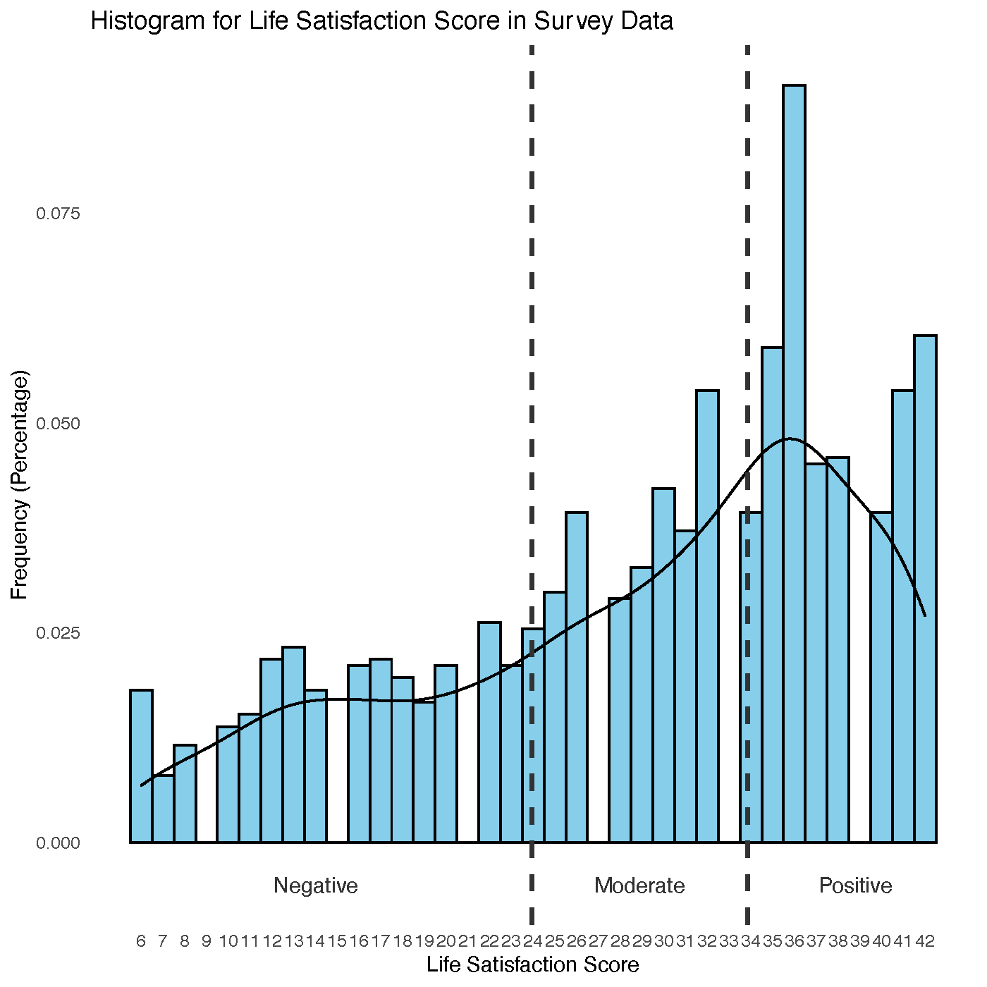
To create the classes I drew the buckets at 0.5 standard deviations away from the mean representing the upper and lower bounds of the “Moderate” life satisfaction. Anything above that would be “Positive”, anything below would be “Negative”. The new distribution of the constructed class is shown below.

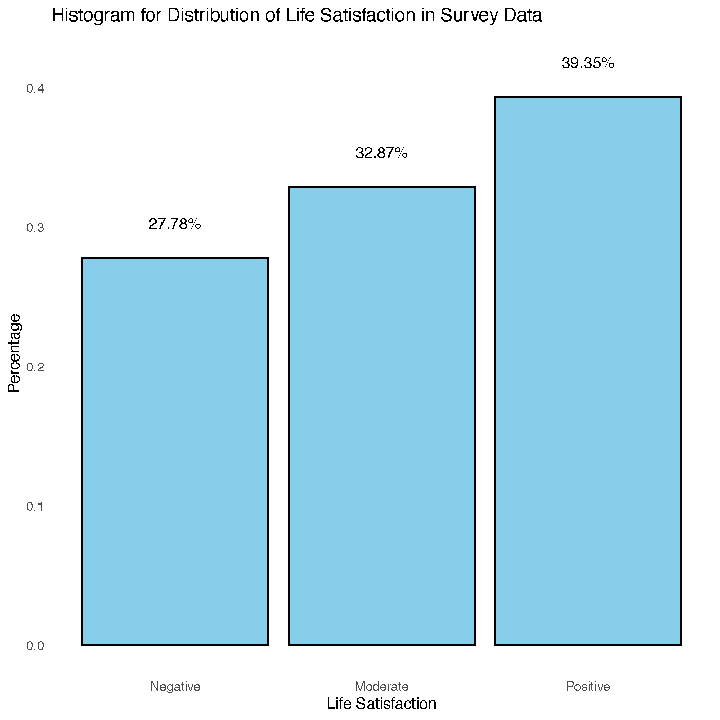
This maintains the skewed distribution present in the life satisfaction score but makes the class distribution manageable for model building and analysis.

The next step was to prune attributes which are either redundant or not-useful for analysis. The survey makers helpfully included a number of “variable with imputation” versions such as with life satisfaction as shown above. These imputation variables corrected for missing data by making a best guess at the values using regression factoring in other attributes in the data set. I elected to keep all variables with imputation and remove their counterparts. In addition I removed the tuple index, population weights (scores used by the survey makers), which survey version was taken, which date the survey was taken, as well as the attributes used to construct the class attribute. Lastly I removed all data which had been hidden by the survey makers to protect the identity of their respondents, since these all contained no data intentionally.

My next step was to prune attributes with too many missing values. If the column had more than 10% NA, intentionally missing values (as defined by the survey makers), or blank (“ “) entries, the entire column was removed. For the remainder of my missing values, I constructed a class-wise mode per attribute and replaced any remaining missing values with the mode of the class for that attribute. This single step imputation is not particularly accurate nor sophisticated, but it is sufficient for my purposes. The last bit of data transformation I did is z-score normalize all numerical columns to eliminate scale, and use a feature of R to coerce all the categorical variable responses into more interpretable variable names for various R functions.

The last step of the data cleaning process was to remove redundant columns in the categorical data. I knew that the numeric data had no redundancy beyond the imputation variables, but the survey questions were less obvious. This was accomplished by doing a pair-wise chi-squared test for independence between every potential pair of columns in the data. With R's chisq.test function, when two columns have identical data it gives a p-value of exactly 0 as opposed to a very low or nearly zero number. I collected these identical column pairs and removed one of each pair to ensure less redundancy in the data.

In the end, the cleaned survey data has 1375 tuples with 201 explanatory variables for the class I am looking to predict. At this stage the data was also split into testing (34%) and training (66%) sets for model building, maintaining the same class ratio as in the survey data.

Initial Model Building And Assessment

I elected to build 5 models for consideration: J48, Random Forest, KNN, Naive Bayes, and Multinomial Logistic. For the initial models, each model was fitted using 10-fold cross validation on the entire set of cleaned survey data using the R library caret to incorporate some hyperparameter tuning to improve overall accuracy.

The assessment tables and visualizations below were constructed using data collected during the cross-validation process, as each fold of data was tested against it's training counterpart, the test set was collected into a performance set to give me a rough idea of how my models would perform against similar, novel data. In theory these models have more data than my feature reduced models and so I would expect a relatively high performance.

Because I have 3 possible classes, each of my performance metrics (except for overall accuracy) is broken down into a class-wise, one-vs-all statistic.

Summary Statistics Table

Model	Reduction	Class	Accuracy	TP Rate	FP Rate	Precision	Recall	F-measure	ROC area	MCC
J48	Nothing	Negative	0.5905	0.5969	0.1138	0.6686	0.5969	0.6307	0.7433	0.5010
J48	Nothing	Moderate	0.5905	0.4580	0.2579	0.4652	0.4580	0.4615	0.5897	0.2009
J48	Nothing	Positive	0.5905	0.6969	0.2542	0.6401	0.6969	0.6673	0.7345	0.4370
J48	Nothing	Weighted Average	0.5905	0.5839	0.2086	0.5913	0.5839	0.5865	0.6892	0.3797
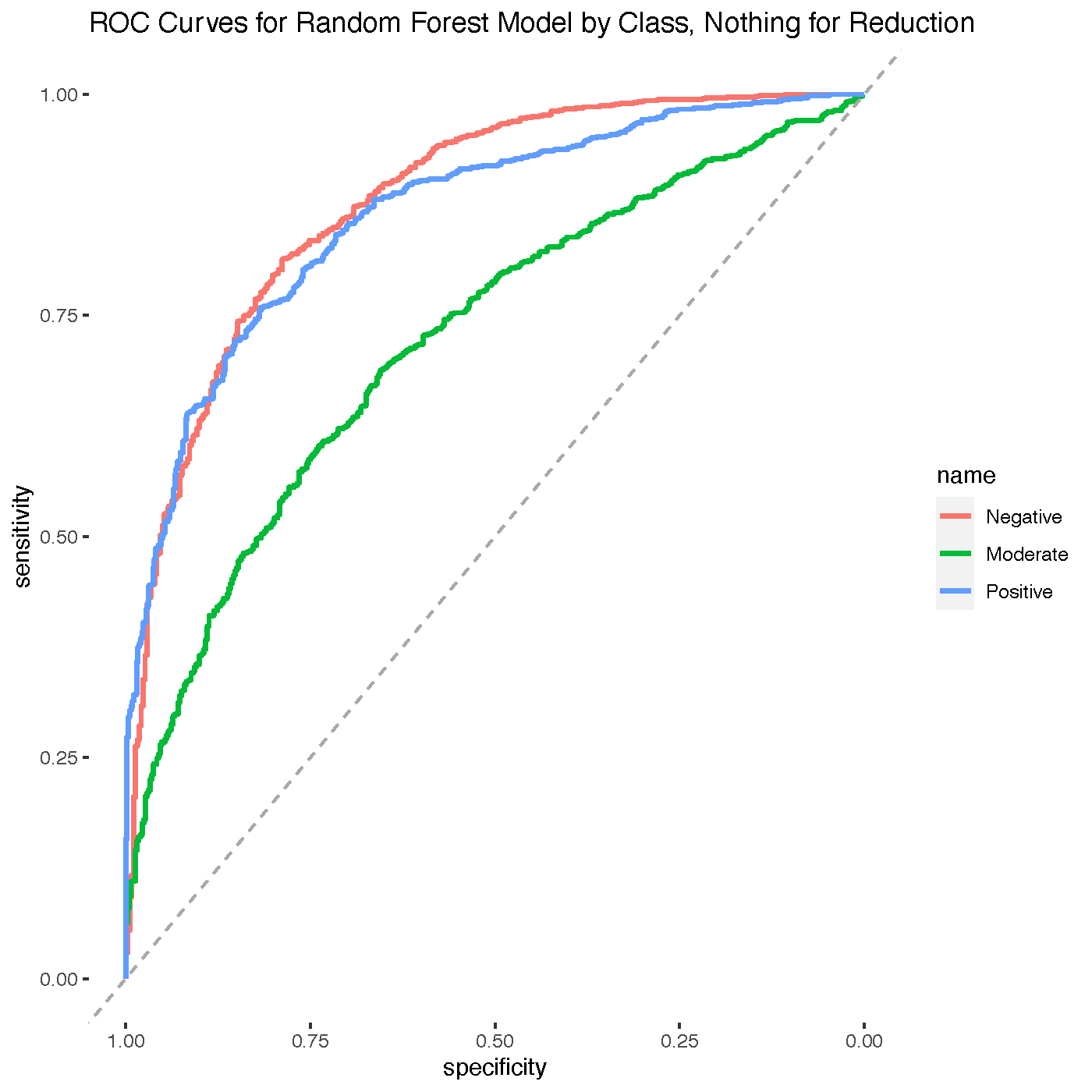
Random Forest	Nothing	Negative	0.6407	0.6518	0.1098	0.6955	0.6518	0.6730	0.8790	0.5533
Random Forest	Nothing	Moderate	0.6407	0.4159	0.1820	0.5281	0.4159	0.4653	0.7221	0.2509
Random Forest	Nothing	Positive	0.6407	0.8207	0.2602	0.6717	0.8207	0.7388	0.8648	0.5480
Random Forest	Nothing	Weighted Average	0.6407	0.6295	0.1840	0.6318	0.6295	0.6257	0.8219	0.4507
KNN	Nothing	Negative	0.5673	0.4607	0.0393	0.8186	0.4607	0.5896	0.8077	0.5198
KNN	Nothing	Moderate	0.5673	0.1969	0.1094	0.4684	0.1969	0.2773	0.6192	0.1191
KNN	Nothing	Positive	0.5673	0.9519	0.5456	0.5309	0.9519	0.6817	0.8177	0.4355
KNN	Nothing	Weighted Average	0.5673	0.5365	0.2314	0.6060	0.5365	0.5162	0.7482	0.3581
Naive Bayes	Nothing	Negative	0.5665	0.5131	0.0937	0.6782	0.5131	0.5842	0.8328	0.4611
Naive Bayes	Nothing	Moderate	0.5665	0.3075	0.2102	0.4174	0.3075	0.3541	0.6169	0.1067
Naive Bayes	Nothing	Positive	0.5665	0.8207	0.3705	0.5896	0.8207	0.6862	0.7748	0.4419
Naive Bayes	Nothing	Weighted Average	0.5665	0.5471	0.2248	0.5618	0.5471	0.5415	0.7415	0.3366
Logistic	Nothing	Negative	0.5709	0.5969	0.1460	0.6113	0.5969	0.6040	0.8170	0.4542
Logistic	Nothing	Moderate	0.5709	0.4425	0.2752	0.4405	0.4425	0.4415	0.6319	0.1671
Logistic	Nothing	Positive	0.5709	0.6599	0.2290	0.6515	0.6599	0.6556	0.8062	0.4299
Logistic	Nothing	Weighted Average	0.5709	0.5664	0.2167	0.5677	0.5664	0.5670	0.7517	0.3504

Each column above has been color coded by class-wise min and max, where green represents the maximum and red the minimum per class, except for FP-Rate where red represents the maximum per class and green represents the minimum.

At a glance we can learn a few things- Naive Bayes is my worst overall performer with a 56.65% accuracy. This makes sense given that the nature of the TransPop survey means a lot of questions are going to be correlated with each other, so the fundamental assumption of naive bayes will be violated. My KNN model clearly is overfitting to the skewed data, preferring to assume most tuples are positive. Logistic and J48 are both underperforming though in different ways- J48 is performing okay at class-wise TP-rate, FP-Rate, precision, and recall but is not as robust as Random Forest, especially for overall assessments like F-score, MCC, and ROC-area. Logistic is okay overall but is not competitive with Random Forest. Random Forest is my undisputed best overall model here, with no class-wise minimum performers and several class-wise maximum performers, including the overall summary statistics.